This tutorial walks you through training a normalizing flow by gradient descent when data is unavailable, but an energy function U(x) proportional to the density p(x) is available.
Setup
import matplotlib.pyplot as plt
import torch

from torch import Tensor

import zuko

_ = torch.random.manual_seed(0)
Energy Function
We consider a simple multi-modal energy function:
logU(x)=sin(πx1)−2(x12+x22−2)2
def log_energy(x: Tensor) -> Tensor:
    x1, x2 = x[..., 0], x[..., 1]
    return torch.sin(torch.pi * x1) - 2 * (x1**2 + x2**2 - 2) ** 2
Visualizing the Energy
Let’s visualize the energy landscape:
x1 = torch.linspace(-3, 3, 64)
x2 = torch.linspace(-3, 3, 64)

x = torch.stack(torch.meshgrid(x1, x2, indexing="xy"), dim=-1)

energy = log_energy(x).exp()
plt.figure(figsize=(4.8, 4.8))
plt.imshow(energy)
plt.show()
Flow
We use a neural spline flow (NSF) as density estimator qϕ(x). However, we invert the transformation(s), which makes sampling more efficient as the inverse call of an autoregressive transformation is D (where D is the number of features) times slower than its forward call.
flow = zuko.flows.NSF(features=2, transforms=3, hidden_features=(64, 64))
flow = zuko.flows.Flow(flow.transform.inv, flow.base)
flow
Inverting the transformation makes sampling more efficient but may make likelihood evaluation slower. This is a good trade-off when training with the reverse KL divergence.
Objective
The objective is to minimize the Kullback-Leibler (KL) divergence between the modeled distribution qϕ(x) and the true data distribution p(x).
argϕmin=argϕmin=argϕmin KL(qϕ(x)∣∣p(x)) Eqϕ(x)[logp(x)qϕ(x)] Eqϕ(x)[logqϕ(x)−logU(x)]
Note that this “reverse KL” objective is prone to mode collapses, especially for high-dimensional data.
Training
optimizer = torch.optim.Adam(flow.parameters(), lr=1e-3)

for epoch in range(8):
    losses = []

    for _ in range(256):
        x, log_prob = flow().rsample_and_log_prob((256,))  # faster than rsample + log_prob

        loss = log_prob.mean() - log_energy(x).mean()
        loss.backward()

        optimizer.step()
        optimizer.zero_grad()

        losses.append(loss.detach())

    losses = torch.stack(losses)

    print(f"({epoch})", losses.mean().item(), "±", losses.std().item())
(0) -0.8076444268226624 ± 1.4574381113052368
(1) -1.5428426265716553 ± 0.1310734897851944
(2) -1.5719032287597656 ± 0.04953986406326294
(3) -1.5784311294555664 ± 0.022914621978998184
(4) -1.5850317478179932 ± 0.023105977103114128
(5) -1.5861082077026367 ± 0.022541742771863937
(6) -1.5803889036178589 ± 0.14612749218940735
(7) -1.5888274908065796 ± 0.017613010480999947
The rsample_and_log_prob method is more efficient than calling rsample and log_prob separately.
Sampling
After training, we can sample from the learned distribution:
samples = flow().sample((16384,))

plt.figure(figsize=(4.8, 4.8))
plt.hist2d(*samples.T, bins=64, range=((-3, 3), (-3, 3)))
plt.show()
Key Differences
The key differences between forward KL (train from data) and reverse KL (train from energy) are:
Data vs Energy
Forward KL requires access to data samples, while reverse KL only needs an energy function.
Mode Coverage
Forward KL tends to cover all modes but may spread probability mass thinly. Reverse KL may miss some modes but concentrates on the main ones.
Sampling Efficiency
Reverse KL benefits from inverting transformations to make sampling more efficient.